6. 表面法向量与多物体
6.1. 基于表面法向量的着色
首先,让我们获取一个表面法向量以进行着色。法向量是垂直于相交点表面的向量。
在代码中,我们需要为法向量做出一个关键的设计决策:法向量可以拥有任意长度,还是应该被归一化为单位长度?
我们倾向于避免计算归一化时昂贵的开平方根运算,以防后续不需要它。然而在实践中,有三个重要的观察结果:第一,如果后续任何地方需要用到单位长度的法向量,你最好一开始就把它处理好,而不是在每个需要它的地方“以防万一”地重复计算。第二,我们在好几个地方确实需要单位长度的法向量。第三,如果你要求法向量必须是单位长度,你通常可以利用对特定几何体类的了解,在它的构造函数或 hit() 函数中高效地生成该向量。例如,球体的法向量只需要直接除以球体半径就能变成单位长度,从而完全避免了开平方根运算。
基于以上原因,我们採取统一策略:所有法向量都将保持单位长度。
对于球体来说,向外的法向量方向是交点减去球心:
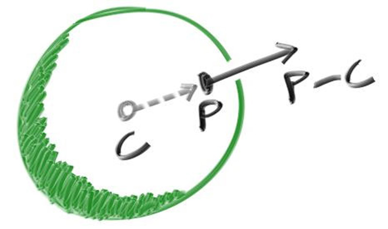
以地球为例,这意味着向量从地心只向你所在的位置,直指你的上方。现在让我们把这个逻辑加入到代码中,并对其进行着色。我们目前还没有加入任何光源之类的东西,所以先单纯地利用颜色映射(Color Map)来将法向量可视化。在可视化法向量时,有一个非常常用的技巧(因为这很容易,而且直观上我们可以假设 是一个单位长度向量,也就是说它的每个分量都在 −1 到 1 之间):将每个分量映射到 0 到 1 的区间内,然后将 对应到 。为了计算常规的法向量,我们需要获取精确的相交点(Hit Point),而不仅仅是像目前这样只判断 “是否相交” 。由于目前场景中只有一个球体,且它正好位于相机的正前方,因此我们暂时先不用担心负的 t 值。我们只需直接假设最近的交点(最小的 t)就是我们想要的那个点。通过对代码进行这些修改,我们就能够计算并将 可视化出来:
double hit_sphere(const point3& center, double radius, const ray& r) {
    vec3 oc = center - r.origin();
    auto a = dot(r.direction(), r.direction());
    auto b = -2.0 * dot(r.direction(), oc);
    auto c = dot(oc, oc) - radius*radius;
    auto discriminant = b*b - 4*a*c;

    if (discriminant < 0) {
        return -1.0;
    } else {
        return (-b - std::sqrt(discriminant) ) / (2.0*a);
    }
}

color ray_color(const ray& r) {
    auto t = hit_sphere(point3(0,0,-1), 0.5, r);
    if (t > 0.0) {
        vec3 N = unit_vector(r.at(t) - vec3(0,0,-1));
        return 0.5*color(N.x()+1, N.y()+1, N.z()+1);
    }

    vec3 unit_direction = unit_vector(r.direction());
    auto a = 0.5*(unit_direction.y() + 1.0);
    return (1.0-a)*color(1.0, 1.0, 1.0) + a*color(0.5, 0.7, 1.0);
}
然后会产出这张图片:

6.2. 化简射线与球体求交代码
让我们重新审视一下射线与球体求交函数:
double hit_sphere(const point3& center, double radius, const ray& r) {
    vec3 oc = center - r.origin();
    auto a = dot(r.direction(), r.direction());
    auto b = -2.0 * dot(r.direction(), oc);
    auto c = dot(oc, oc) - radius*radius;
    auto discriminant = b*b - 4*a*c;

    if (discriminant < 0) {
        return -1.0;
    } else {
        return (-b - std::sqrt(discriminant) ) / (2.0*a);
    }
}
首先,回想一下,一个向量与自己做内积等于该向量长度的平方。
其次,请注意 的方程中包含一个 −2 的因子。让我们考虑一下,如果令 ,一元二次方程会发生怎样的变化:
这很好的化简了式子,所以我们将使用它。求解 的表达式为:
使用以上观察,我们可以将射线与球体求交代码化简如下:
double hit_sphere(const point3& center, double radius, const ray& r) {
    vec3 oc = center - r.origin();
    auto a = r.direction().length_squared();
    auto h = dot(r.direction(), oc);
    auto c = oc.length_squared() - radius*radius;
    auto discriminant = h*h - a*c;

    if (discriminant < 0) {
        return -1.0;
    } else {
        return (h - std::sqrt(discriminant)) / a;
    }
}
6.3. 可击中物体的抽象化
现在,如果是多个球体的情况呢?虽然我们很容易倾向直接使用一个球体数组,但更乾淨的做法是为光线可能击中的任何几何体创建一个 “抽象类(Abstract Class)” ,并将 ”单个球体“ 和 “球体列表” 都统一视为可以被光线击中的对象。给这个类起什么名字着实让人有些犯难——如果不是因为“面向对象(Object-Oriented)”编程中已经有了这个词,使用 “对象(object)” 会是个不错的选择。 “表面(surface)” 也很常用,但缺点是未来我们可能想引入体积(雾、云,或类似的东西)而 “可击中(hittable)“ 这个名字突出了将它们统一在一起的核心成员函数。虽然这些名字我都不算最满意,但我们会使用 ”可击中“ 。
这个名为 hittable 的抽象类将包含一个接收光线的 hit 函数。大多数光线追踪器的开发者都发现,为交点引入一个有效区间 会非常方便,也就是说,只有当 时,这次相交才算真正有效。对于最初发射的射线(主射线),这个区间通常是正数 t。但正如我们随后看到的,定义一个区间 可以大大简化我们的代码。另一个架构设计问题是,如果我们击中了某个物体,是否应该立即计算表面法向量等信息?因为在遍历场景的过程中,我们随后可能会击中一个更近的物体,因此我们最终只需要那个最近物体的法向量。在这里,我将採用最简单的解决方案,将所有计算出的一捆信息(交点、法线等)打包存储到某个结构体(Structure)中。以下是这个抽象类的定义:
#ifndef HITTABLE_H
#define HITTABLE_H

#include "ray.h"

class hit_record {
  public:
    point3 p;
    vec3 normal;
    double t;
};

class hittable {
  public:
    virtual ~hittable() = default;

    virtual bool hit(const ray& r, double ray_tmin, double ray_tmax, hit_record& rec) const = 0;
};

#endif
然后这是球体:
#ifndef SPHERE_H
#define SPHERE_H

#include "hittable.h"
#include "vec3.h"

class sphere : public hittable {
  public:
    sphere(const point3& center, double radius) : center(center), radius(std::fmax(0,radius)) {}

    bool hit(const ray& r, double ray_tmin, double ray_tmax, hit_record& rec) const override {
        vec3 oc = center - r.origin();
        auto a = r.direction().length_squared();
        auto h = dot(r.direction(), oc);
        auto c = oc.length_squared() - radius*radius;

        auto discriminant = h*h - a*c;
        if (discriminant < 0)
            return false;

        auto sqrtd = std::sqrt(discriminant);

        // 寻找可接受范围内最近的根
        auto root = (h - sqrtd) / a;
        if (root <= ray_tmin || ray_tmax <= root) {
            root = (h + sqrtd) / a;
            if (root <= ray_tmin || ray_tmax <= root)
                return false;
        }

        rec.t = root;
        rec.p = r.at(rec.t);
        rec.normal = (rec.p - center) / radius;

        return true;
    }

  private:
    point3 center;
    double radius;
};

#endif
(注意,这里我们使用了 C++ 标准库函数 std::fmax(),它会返回两个浮点数参数中的较大值。同理,我们稍后还会用到 std::fmin(),它会返回两个浮点数参数中的较小值。)
6.4. 正面与背面
法向量的第二个设计决策是,它是否永远指向外部(朝外)。目前,我们求得的法线方向始终是从球心指向交点(法向量朝外)。如果光线从外部与球体相交,法线方向与光线方向相反;如果光线从内部与球体相交,法线(依然朝外)方向则与光线方向相同。另一种替代方案是,我们可以让法线始终逆着光线的方向。如果光线在球体外部,法线将朝外;但如果光线在球体内部,法线将转为朝内。
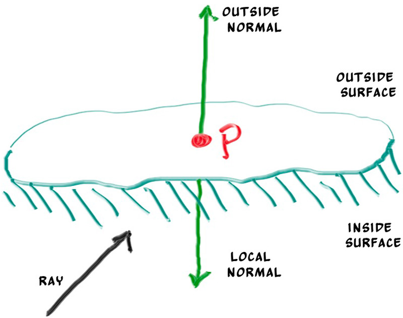
我们需要选择其中一个可能性,因为我们最终需要确定射线来自表面的哪一面。这对两侧渲染方式不同的物体很重要,像是纸张两面的文字,或者有分内侧外侧的物体,像是玻璃球。
如果我们决定让法向量永远朝外,则进行着色时,我们需要判断射线位于物体的哪一侧。藉由比较射线和法向量,我们可以得知这一点。若两者同向,则射线在物体内部;若两者反向,则射线在物体外部。这可以透过计算这两个向量的内积来判定,若内积是正数,则射线在物体内部。
if (dot(ray_direction, outward_normal) > 0.0) {
    // 射线在球体内
    ...
} else {
    // 射线在球体外
    ...
}
如果我们决定让法向量永远与射线反向,则我们无法用内积判定射线在表面的哪一面。作为替代,我们需要存储这一资讯。
bool front_face;
if (dot(ray_direction, outward_normal) > 0.0) {
    // 射线在球体内
    normal = -outward_normal;
    front_face = false;
} else {
    // 射线在球体外
    normal = outward_normal;
    front_face = true;
}
我们可以进行设置,使法向量永远从表面指向外部,或者总是逆着入射光线的方向。这取决于你想要在几何体相交之时,还是在进行着色之时来确定表面在哪一侧。在本书中,我们拥有的材质类型多于几何体类型,因此我们选择做更少工作的方式,将此判定放在几何体相交之时。这纯粹是一个偏好问题,你在文献中会看到这两种实作方式。
我们将 front_face 布尔值添加到 hit_record 类中。我们再添加一个函数来为我们解决这个计算:set_face_normal()。为了方便起见,我们假设传递给新 set_face_normal() 函数的向量是单位长度。我们总是可以显式地将该参数进行归一化,但如果由几何体代码来做这件事会更有效率,因为当你对特定几何体了解更多时,这通常会更容易。
class hit_record {
  public:
    point3 p;
    vec3 normal;
    double t;
    bool front_face;

    void set_face_normal(const ray& r, const vec3& outward_normal) {
        // 设置撞击记录的法向量。
        // 注意:参数 outward_normal 被假定为单位长度。

        front_face = dot(r.direction(), outward_normal) < 0;
        normal = front_face ? outward_normal : -outward_normal;
    }
};
然后我们将表面两侧的判定添加到该类中:
class sphere : public hittable {
  public:
    ...
    bool hit(const ray& r, double ray_tmin, double ray_tmax, hit_record& rec) const {
        ...

        rec.t = root;
        rec.p = r.at(rec.t);
        vec3 outward_normal = (rec.p - center) / radius;
        rec.set_face_normal(r, outward_normal);

        return true;
    }
    ...
};
6.5. 可碰撞物体的列表
我们有一个名为 hittable 的通用对象,光线可以与之相交。我们现在添加一个存储 hittables 列表的类:
#ifndef HITTABLE_LIST_H
#define HITTABLE_LIST_H

#include "hittable.h"

#include <memory>
#include <vector>

using std::make_shared;
using std::shared_ptr;

class hittable_list : public hittable {
  public:
    std::vector<shared_ptr<hittable>> objects;

    hittable_list() {}
    hittable_list(shared_ptr<hittable> object) { add(object); }

    void clear() { objects.clear(); }

    void add(shared_ptr<hittable> object) {
        objects.push_back(object);
    }

    bool hit(const ray& r, double ray_tmin, double ray_tmax, hit_record& rec) const override {
        hit_record temp_rec;
        bool hit_anything = false;
        auto closest_so_far = ray_tmax;

        for (const auto& object : objects) {
            if (object->hit(r, ray_tmin, closest_so_far, temp_rec)) {
                hit_anything = true;
                closest_so_far = temp_rec.t;
                rec = temp_rec;
            }
        }

        return hit_anything;
    }
};

#endif
6.6. 一些新的 C++ 特性
hittable_list 类代码中使用了一些 C++ 特性,如果你平时不怎么写 C++,可能会觉得有点陌生:vector、shared_ptr 和 make_shared。
shared_ptr<type> 是一个指向某种已分配内存类型的指针,它具有引用计数语义。每当你把它赋值给另一个智能指针时(通常通过简单的赋值操作),它的引用计数就会加 1。当智能指针超出作用域(例如在代码块或函数结束时),引用计数就会减 1。一旦引用计数归零,该对象就会被安全地自动销毁。
通常情况下,智能指针首先会用一个新分配的对象来进行初始化,代码类似于这样:
shared_ptr<double> double_ptr = make_shared<double>(0.37);
shared_ptr<vec3>   vec3_ptr   = make_shared<vec3>(1.414214, 2.718281, 1.618034);
shared_ptr<sphere> sphere_ptr = make_shared<sphere>(point3(0,0,0), 1.0);
make_shared<thing>(thing_constructor_params ...) 会使用构造函数参数分配一个 thing 类型的新实例。它返回一个 shared_ptr<thing>。
由于通过 make_shared<type>(...) 的返回值可以直接自动推导出来类型,上述代码可以使用 C++ 的 auto 类型说明符来更简洁地表达:
auto double_ptr = make_shared<double>(0.37);
auto vec3_ptr   = make_shared<vec3>(1.414214, 2.718281, 1.618034);
auto sphere_ptr = make_shared<sphere>(point3(0,0,0), 1.0);
我们在代码中会使用智能指针(shared pointers),因为它们允许不同的几何体共享同一个实例(例如,一大群球体都使用同一种颜色的材质),而且它能实现内存自动管理,让逻辑变得更清晰。
std::shared_ptr 包含在 <memory> 头文件中。
你可能不太熟悉的第二个 C++ 特性是 std::vector。这是一个存储任意类型的通用动态数组。在上面,我们使用了一个存储 hittable 指针的集合。随着更多元素的加入,std::vector 会自动扩容:objects.push_back(object) 会将一个元素添加到 std::vector 成员变量 objects 的末尾。
std::vector 包含在 <vector> 头文件中。
最后,代码清单 21 中的 using 声明告诉编译器,我们将从 std 标准库中引入 shared_ptr 和 make_shared,因此在每次引用它们时,都不需要再加上 std:: 前缀。
6.7. 常用常量和工具函数
我们将需要的数学常数方便地定义在它们自己的头文件中。目前只需要无穷大,但我们也会把自己的圆周率定义放进去,这稍后会需要。我们还会把常用的实用常数和未来的工具函数放进这里。这个新的头文件,rtweekend.h,将成为我们的通用主头文件。
#ifndef RTWEEKEND_H
#define RTWEEKEND_H

#include <cmath>
#include <iostream>
#include <limits>
#include <memory>


// C++ 标准库的 using 声明

using std::make_shared;
using std::shared_ptr;

// 常量

const double infinity = std::numeric_limits<double>::infinity();
const double pi = 3.1415926535897932385;

// 工具函数

inline double degrees_to_radians(double degrees) {
    return degrees * pi / 180.0;
}

// 常用头文件

#include "color.h"
#include "ray.h"
#include "vec3.h"

#endif
程序文件将首先包含 rtweekend.h,因此所有其他头文件(我们代码的大部分将存放在那里)都可以隐式地假设 rtweekend.h 已经被包含。头文件仍然需要显式地包含任何其他必要的头文件。我们将记住这些假设并进行一些更新:
#include <iostream>
#include "ray.h"
#include <memory>
#include <vector>

using std::make_shared;
using std::shared_ptr;
#include "vec3.h"
#include <cmath> #include <iostream>
现在新的 main 如下:
#include "rtweekend.h"

#include "color.h"
#include "ray.h"
#include "vec3.h"
#include "hittable.h"
#include "hittable_list.h"
#include "sphere.h"

#include <iostream>

double hit_sphere(const point3& center, double radius, const ray& r) {
    ...
}

color ray_color(const ray& r, const hittable& world) {
   hit_record rec;
   if (world.hit(r, 0, infinity, rec)) {
       return 0.5 * (rec.normal + color(1,1,1));
   }

    vec3 unit_direction = unit_vector(r.direction());
    auto a = 0.5*(unit_direction.y() + 1.0);
    return (1.0-a)*color(1.0, 1.0, 1.0) + a*color(0.5, 0.7, 1.0);
}

int main() {

    // 图像

    auto aspect_ratio = 16.0 / 9.0;
    int image_width = 400;

    // 计算图像的高,并确保它至少为 1。
    int image_height = int(image_width / aspect_ratio);
    image_height = (image_height < 1) ? 1 : image_height;

   // 世界

   hittable_list world;

   world.add(make_shared<sphere>(point3(0,0,-1), 0.5));
   world.add(make_shared<sphere>(point3(0,-100.5,-1), 100));

    // 相机

    auto focal_length = 1.0;
    auto viewport_height = 2.0;
    auto viewport_width = viewport_height * (double(image_width)/image_height);
    auto camera_center = point3(0, 0, 0);

    // 计算视口水平边缘和垂直边缘的向量
    auto viewport_u = vec3(viewport_width, 0, 0);
    auto viewport_v = vec3(0, -viewport_height, 0);

    // 计算相邻像素间水平和垂直间距向量
    auto pixel_delta_u = viewport_u / image_width;
    auto pixel_delta_v = viewport_v / image_height;

    // 计算左上角像素的位置
    auto viewport_upper_left = camera_center
                             - vec3(0, 0, focal_length) - viewport_u/2 - viewport_v/2;
    auto pixel00_loc = viewport_upper_left + 0.5 * (pixel_delta_u + pixel_delta_v);

    // 渲染

    std::cout << "P3\n" << image_width << ' ' << image_height << "\n255\n";

    for (int j = 0; j < image_height; j++) {
        std::clog << "\rScanlines remaining: " << (image_height - j) << ' ' << std::flush;
        for (int i = 0; i < image_width; i++) {
            auto pixel_center = pixel00_loc + (i * pixel_delta_u) + (j * pixel_delta_v);
            auto ray_direction = pixel_center - camera_center;
            ray r(camera_center, ray_direction);

            color pixel_color = ray_color(r, world);
            write_color(std::cout, pixel_color);
        }
    }

    std::clog << "\rDone.                 \n";
}
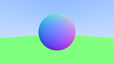
这产生了以下图像,它实际上只是球体所在位置以及它们表面法线的视觉化。这通常是查看几何模型缺陷或特定特徵的极佳方式。
6.8. 一个区间类
在我们继续之前,我们实作一个区间类,以管理一个有最大、最小值的实数区间。随着推进,我们将非常频繁地使用这个类。
#ifndef INTERVAL_H
#define INTERVAL_H

class interval {
  public:
    double min, max;

    interval() : min(+infinity), max(-infinity) {} // 预设区间是空的

    interval(double min, double max) : min(min), max(max) {}

    double size() const {
        return max - min;
    }

    bool contains(double x) const {
        return min <= x && x <= max;
    }

    bool surrounds(double x) const {
        return min < x && x < max;
    }

    static const interval empty, universe;
};

const interval interval::empty    = interval(+infinity, -infinity);
const interval interval::universe = interval(-infinity, +infinity);

#endif
// 常用头文件

#include "color.h"
#include "interval.h"
#include "ray.h"
#include "vec3.h"
class hittable {
  public:
    ...
    virtual bool hit(const ray& r, interval ray_t, hit_record& rec) const = 0;
};
class hittable_list : public hittable {
  public:
    ...
    bool hit(const ray& r, interval ray_t, hit_record& rec) const override {
        hit_record temp_rec;
        bool hit_anything = false;
        auto closest_so_far = ray_t.max;

        for (const auto& object : objects) {
            if (object->hit(r, interval(ray_t.min, closest_so_far), temp_rec)) {
                hit_anything = true;
                closest_so_far = temp_rec.t;
                rec = temp_rec;
            }
        }

        return hit_anything;
    }
    ...
};
class sphere : public hittable {
  public:
    ...
    bool hit(const ray& r, interval ray_t, hit_record& rec) const override {
        ...

        // 寻找可接受范围内最近的根
        auto root = (h - sqrtd) / a;
        if (!ray_t.surrounds(root)) {
            root = (h + sqrtd) / a;
            if (!ray_t.surrounds(root))
                return false;
        }
        ...
    }
    ...
};
color ray_color(const ray& r, const hittable& world) {
    hit_record rec;
    if (world.hit(r, interval(0, infinity), rec)) {
        return 0.5 * (rec.normal + color(1,1,1));
    }

    vec3 unit_direction = unit_vector(r.direction());
    auto a = 0.5*(unit_direction.y() + 1.0);
    return (1.0-a)*color(1.0, 1.0, 1.0) + a*color(0.5, 0.7, 1.0);
}